

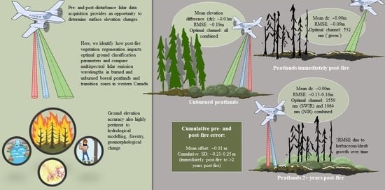
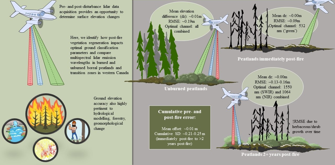
Quantifying Lidar Elevation Accuracy: Parameterization and Wavelength Selection for Optimal Ground Classifications Based on Time since Fire/Disturbance

Abstract
:
1. Introduction
2. Materials and Methods
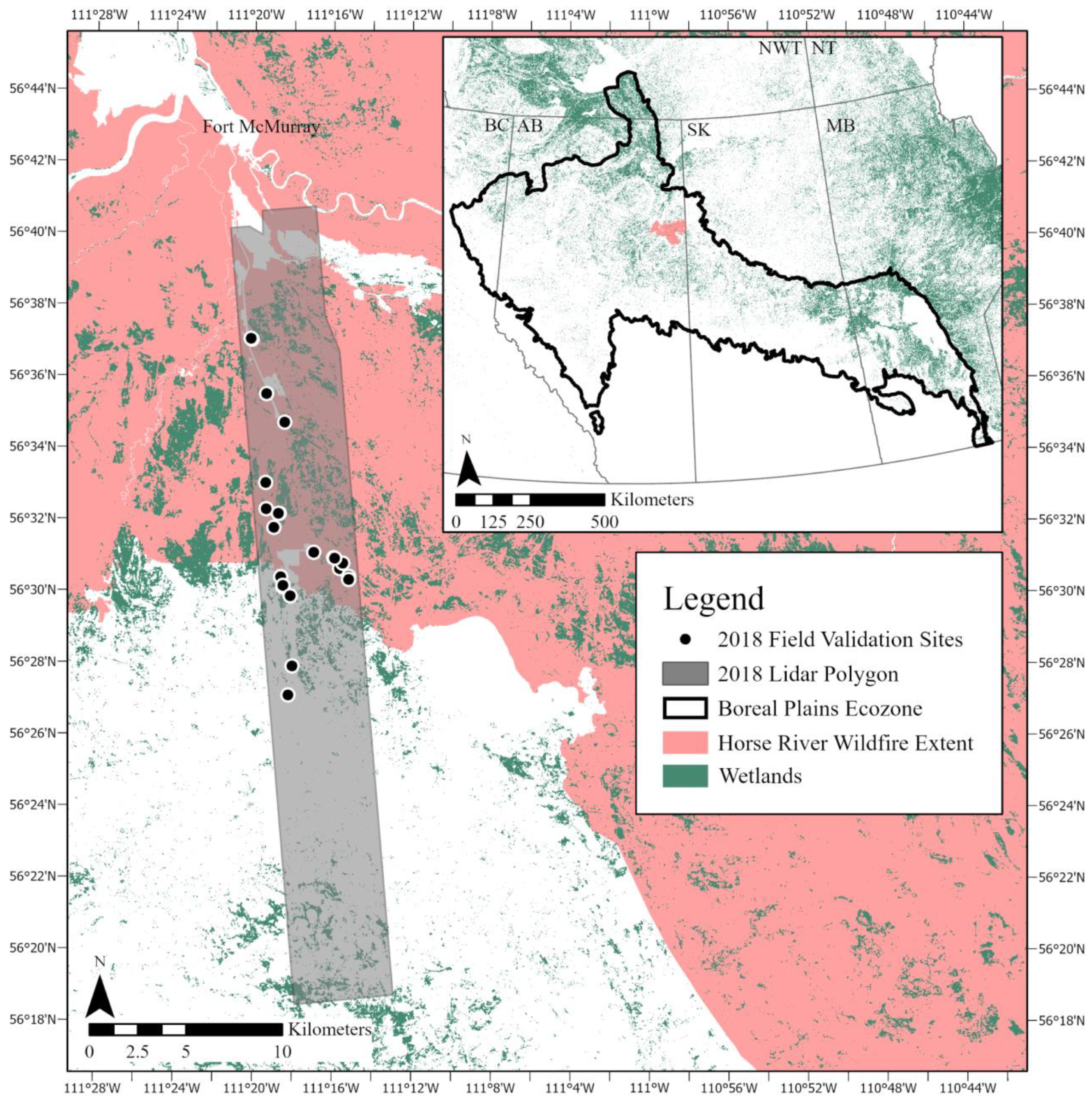
2.1. Study Area
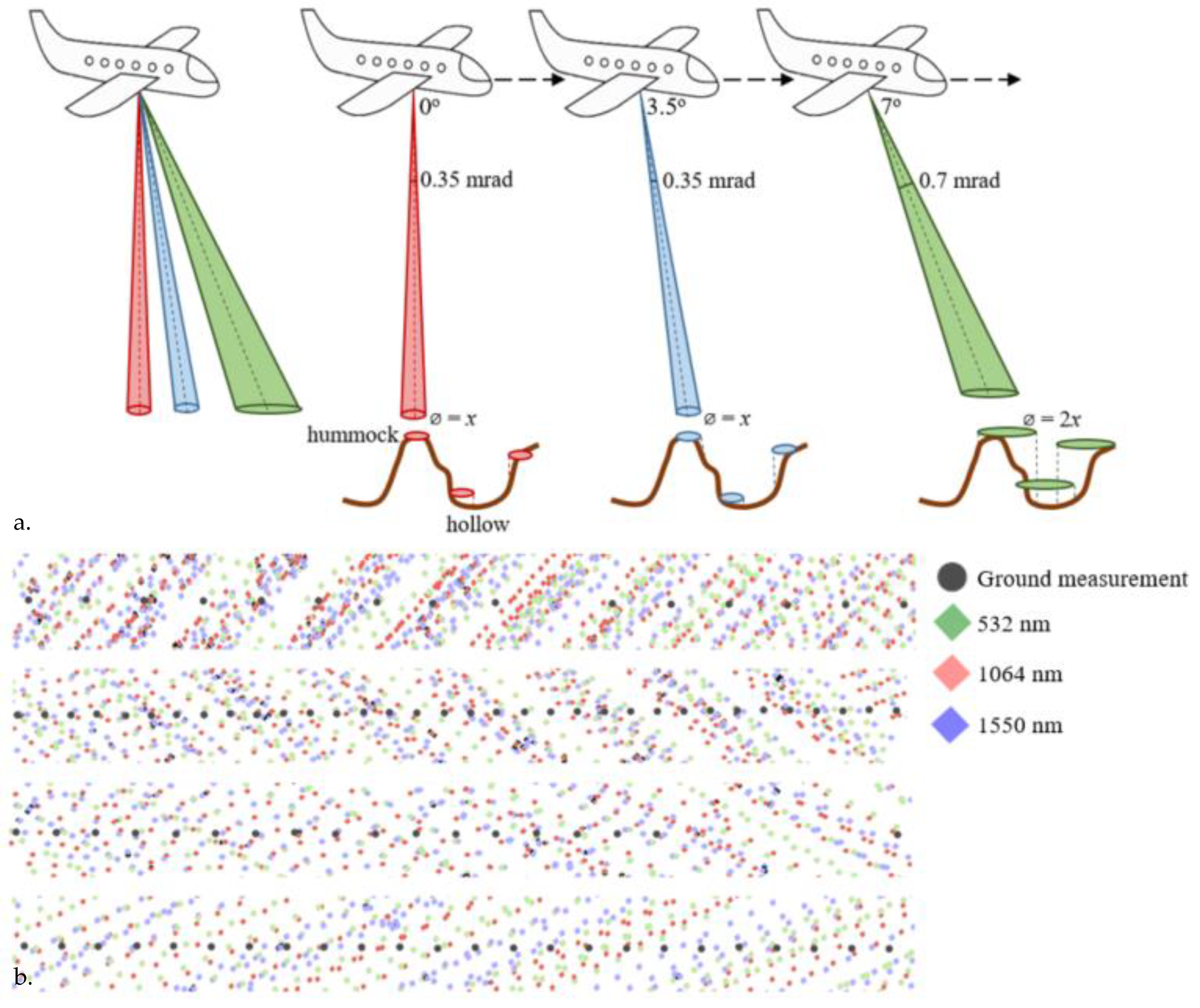
2.2. Data Acquisition
2.3. Data Processing
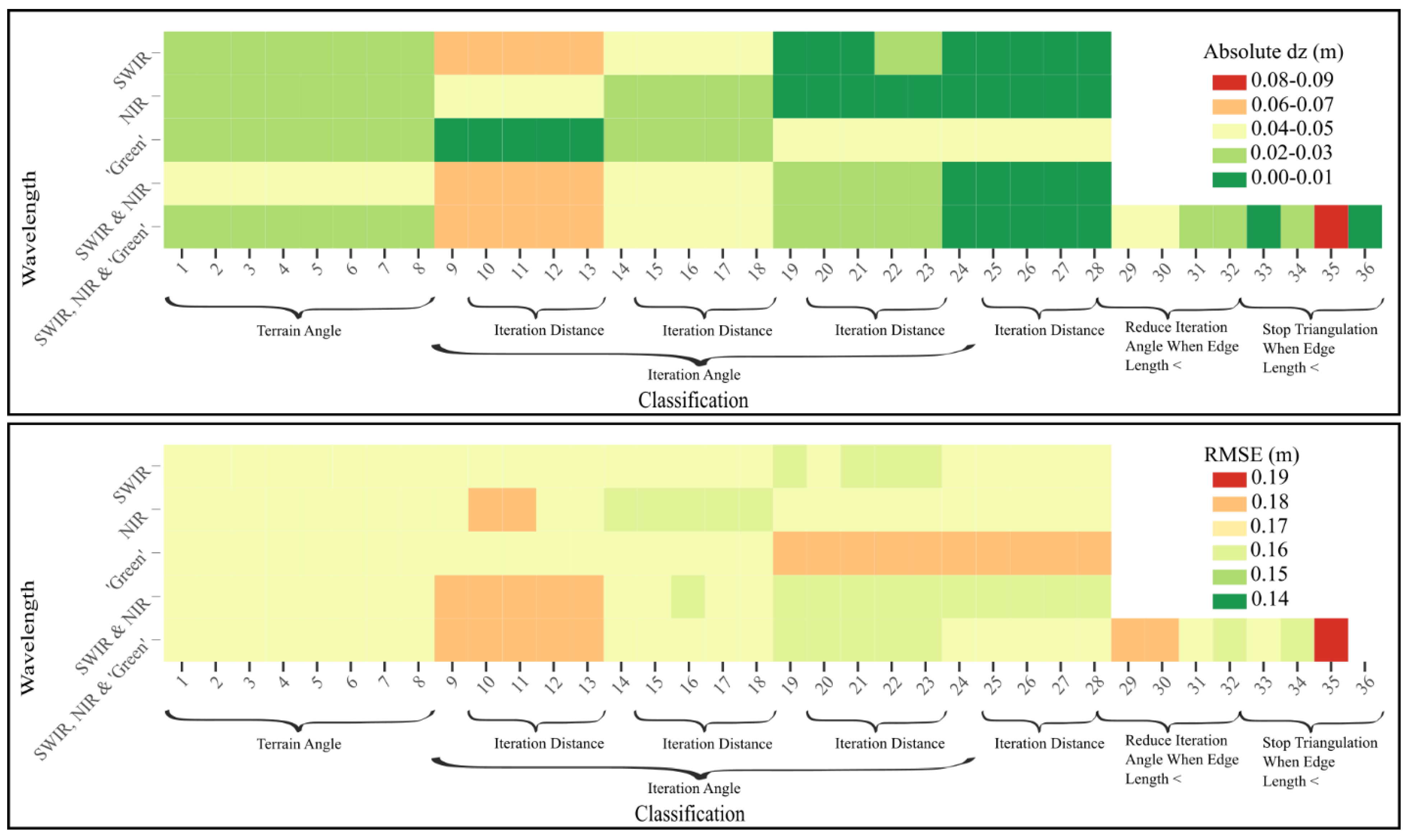
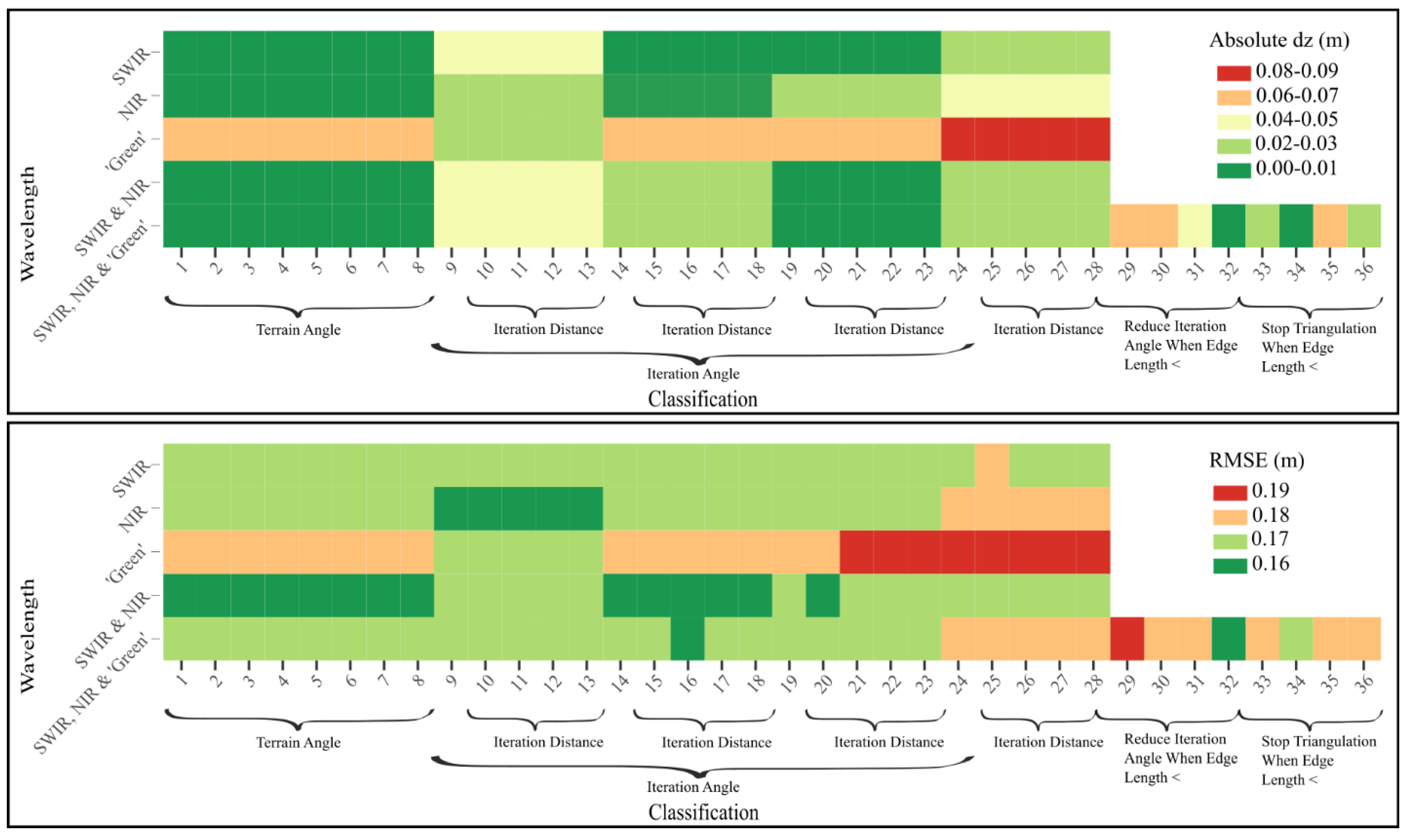
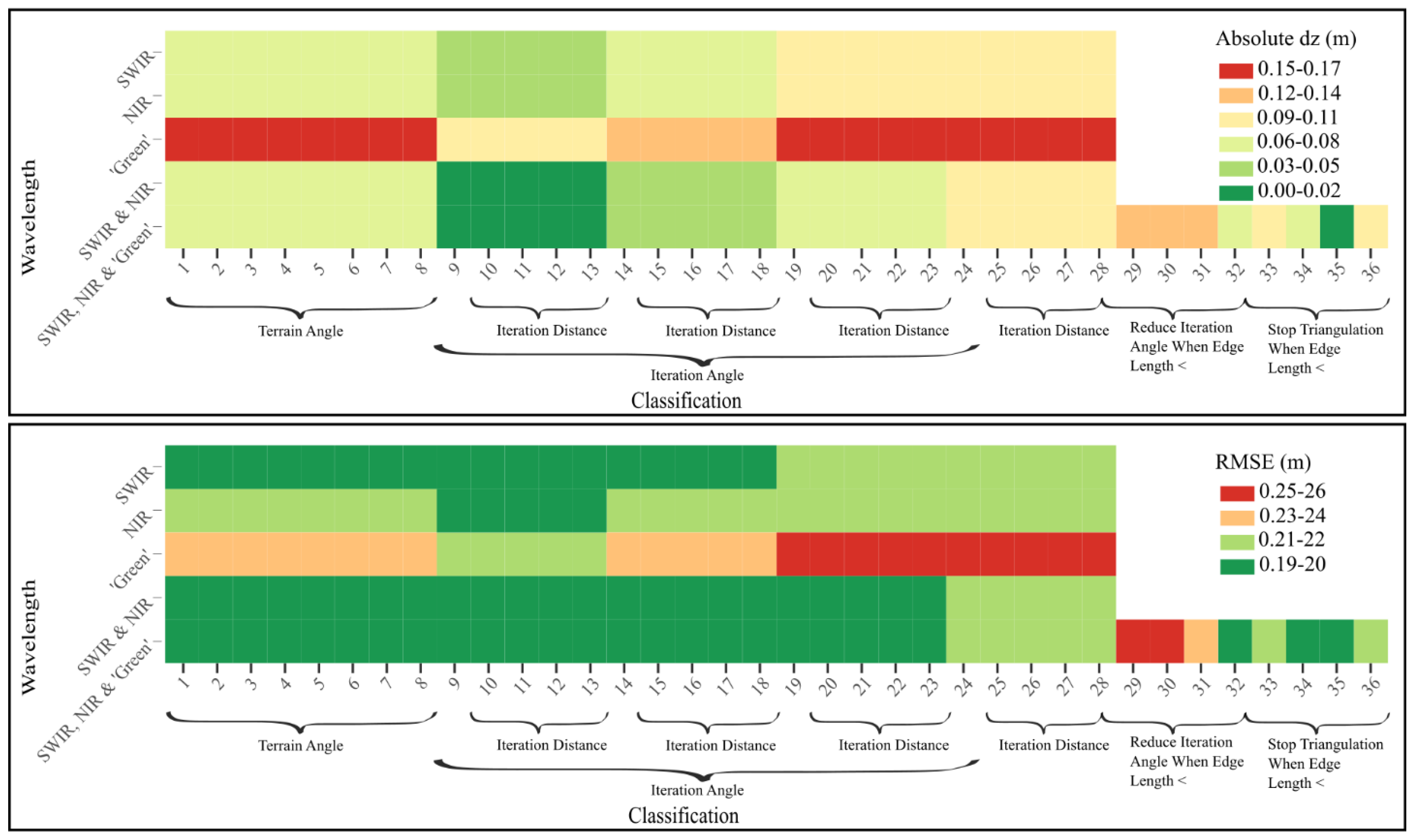
2.3.1. TerraScan
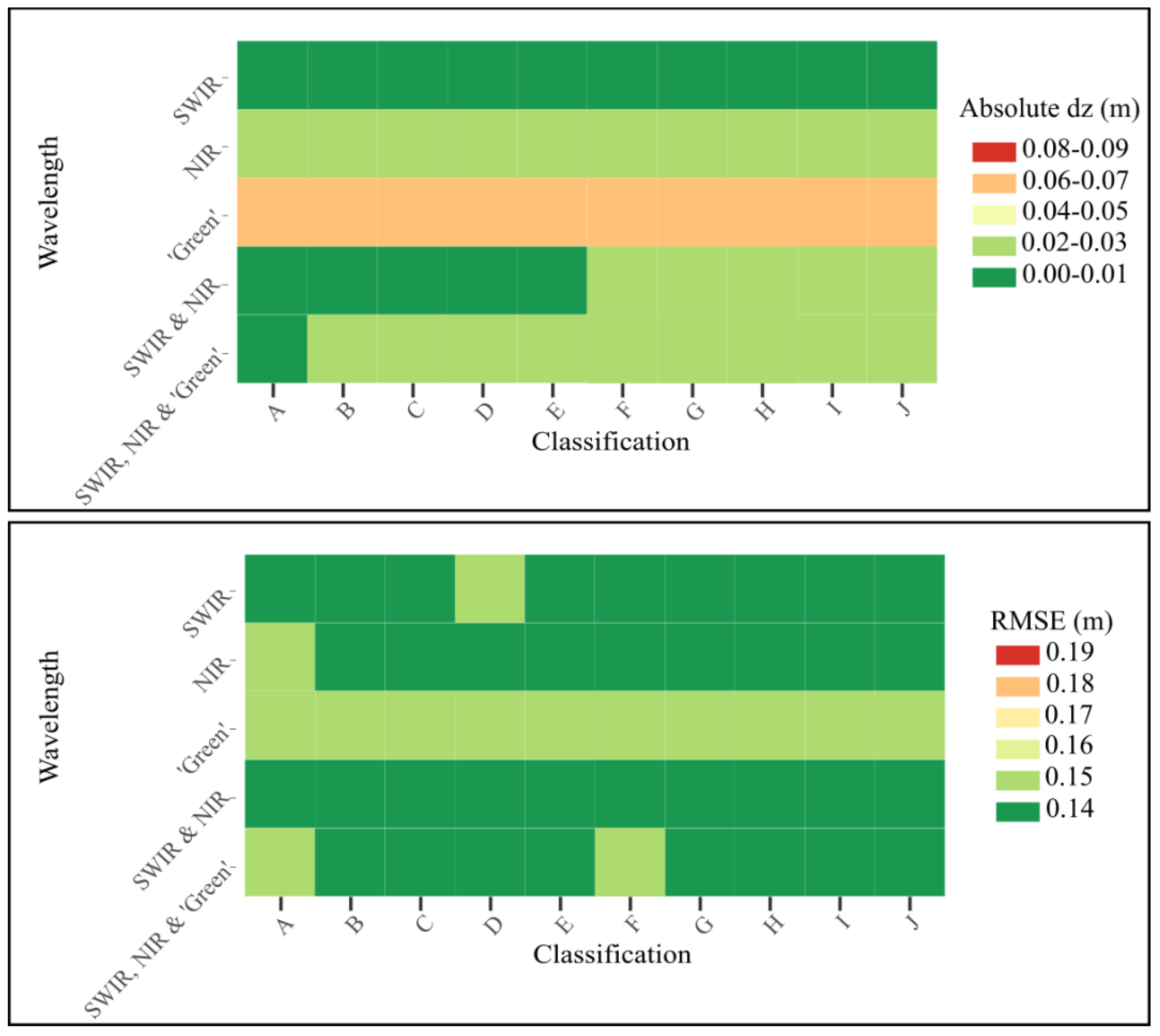
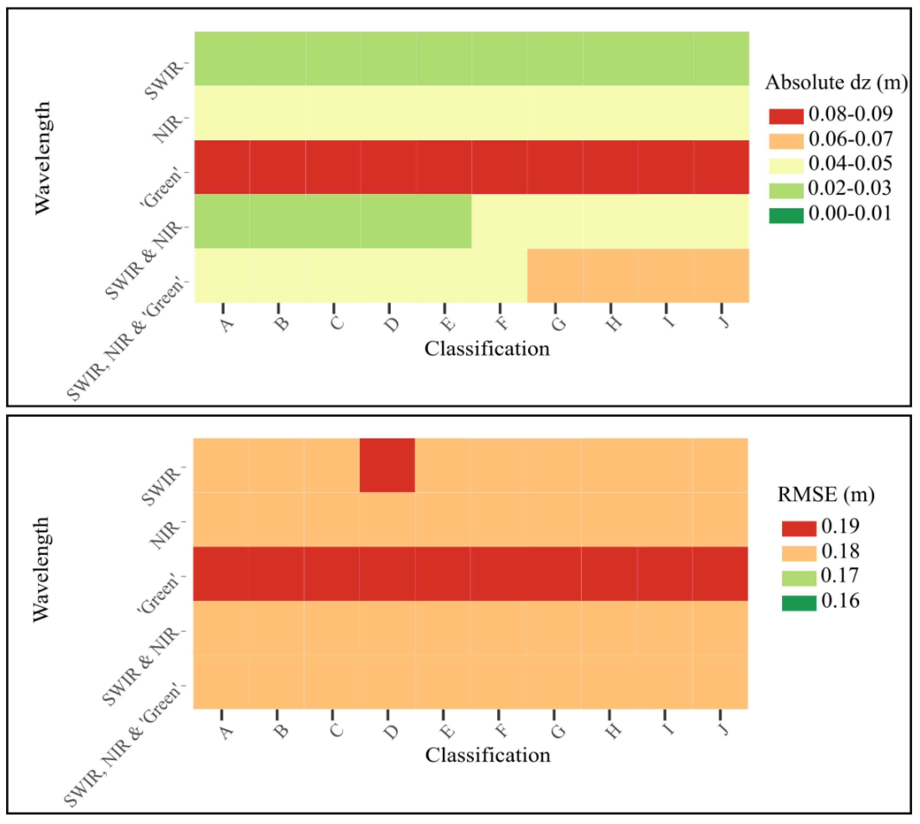
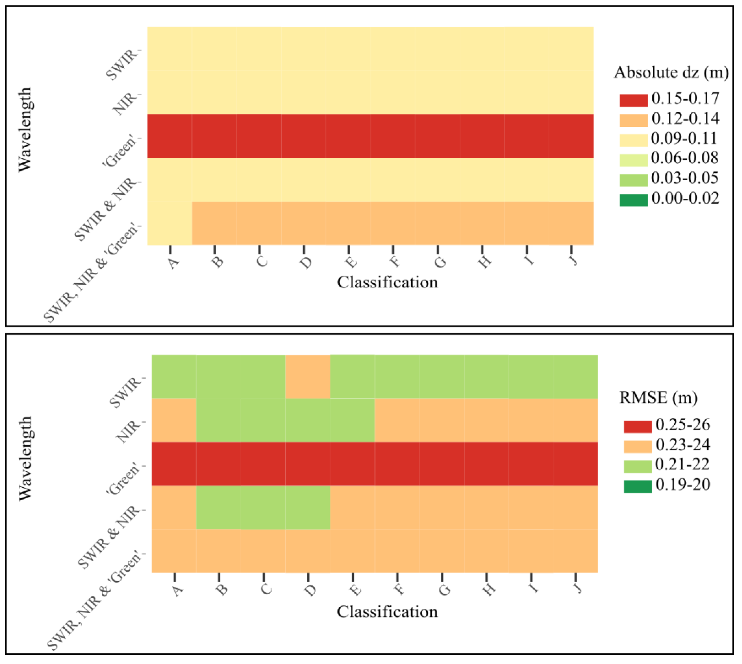
2.3.2. LAStools
2.4. Vertical Accuracy Assessment
3. Results
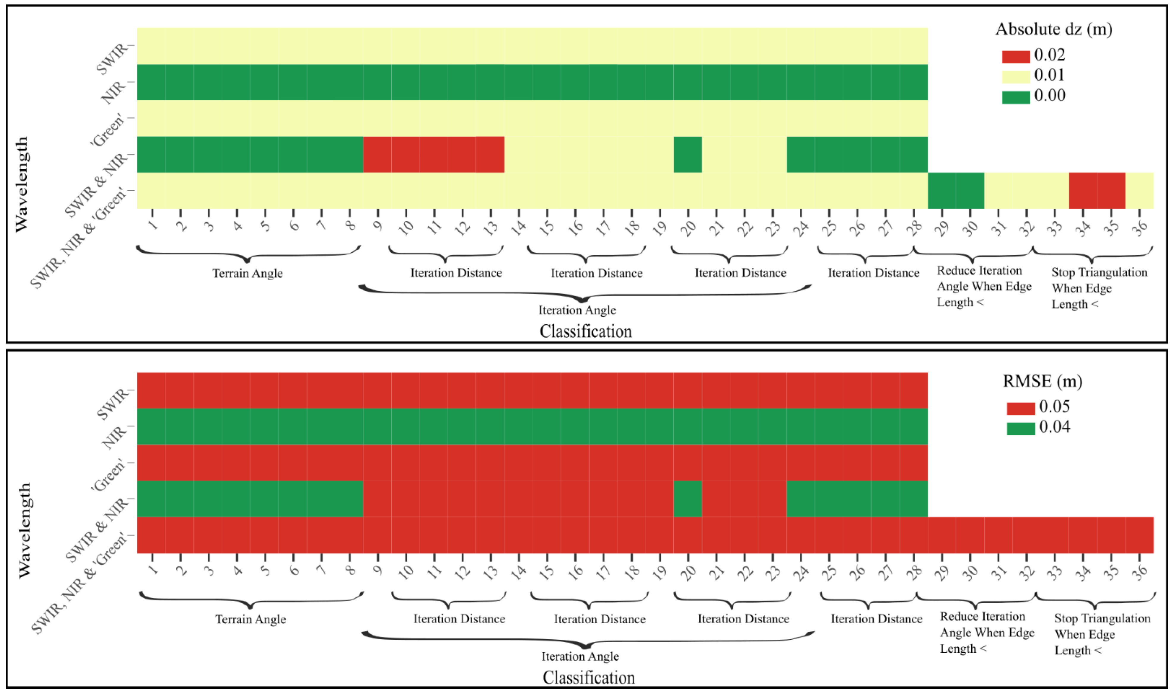
3.1. Differences between Ground-Surveyed Road Elevations and Lidar-Measured Road Ground Classifications
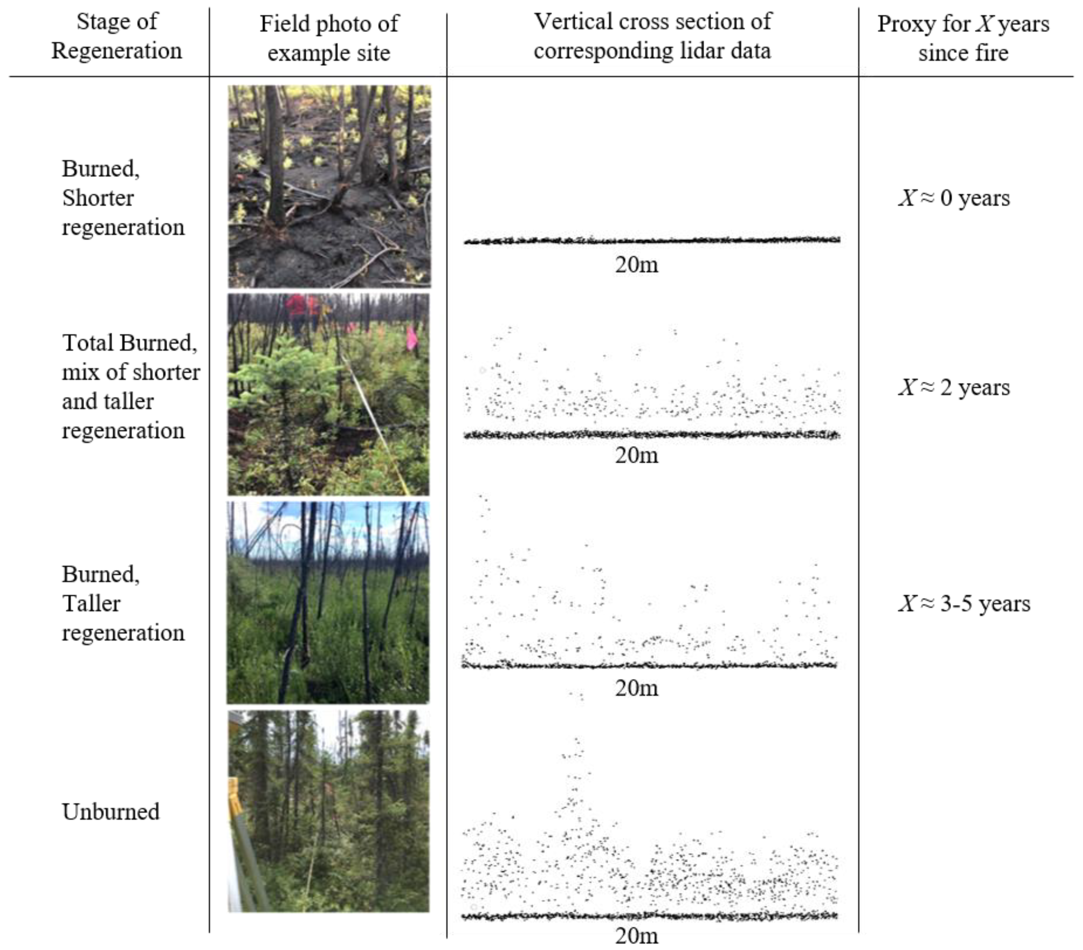
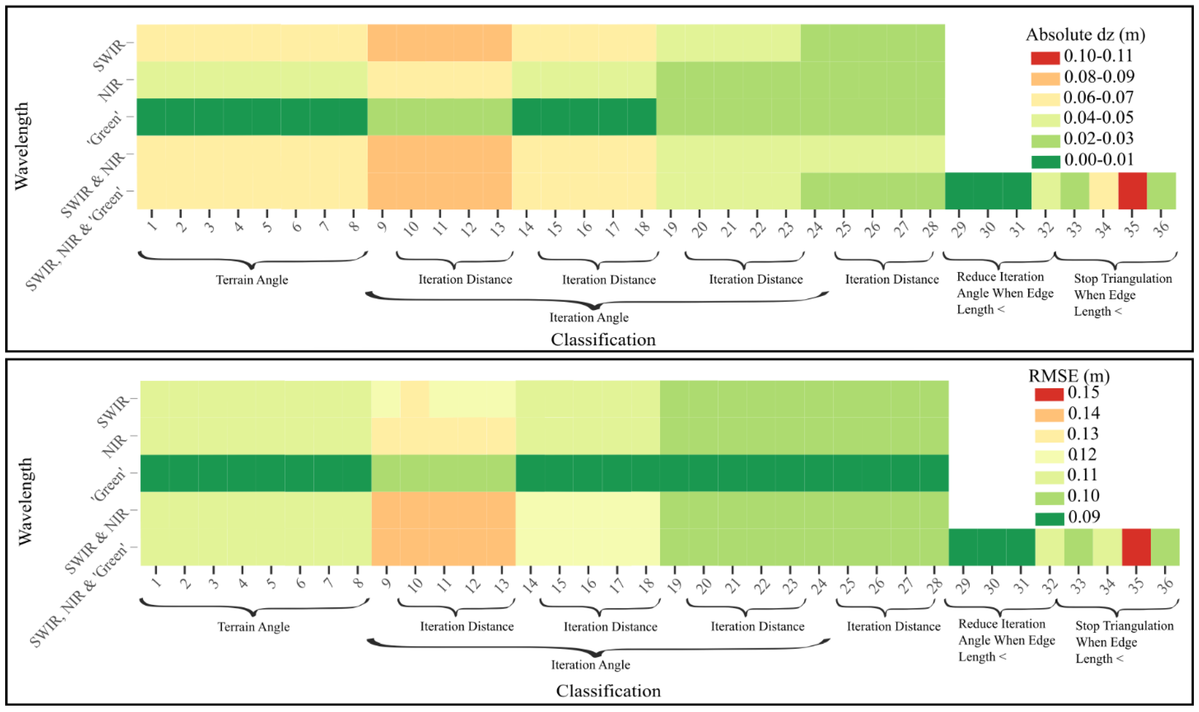
3.2. Differences between Field-Measured Elevation and Lidar Return Ground Classification in Shorter Vegetative Regeneration Peatlands
3.3. Differences between Field-Measured Elevation and Lidar Ground Classification across All Burned Peatlands (Cumulative Shorter Vegetative Regeneration and Taller Vegetative Regeneration Sites)
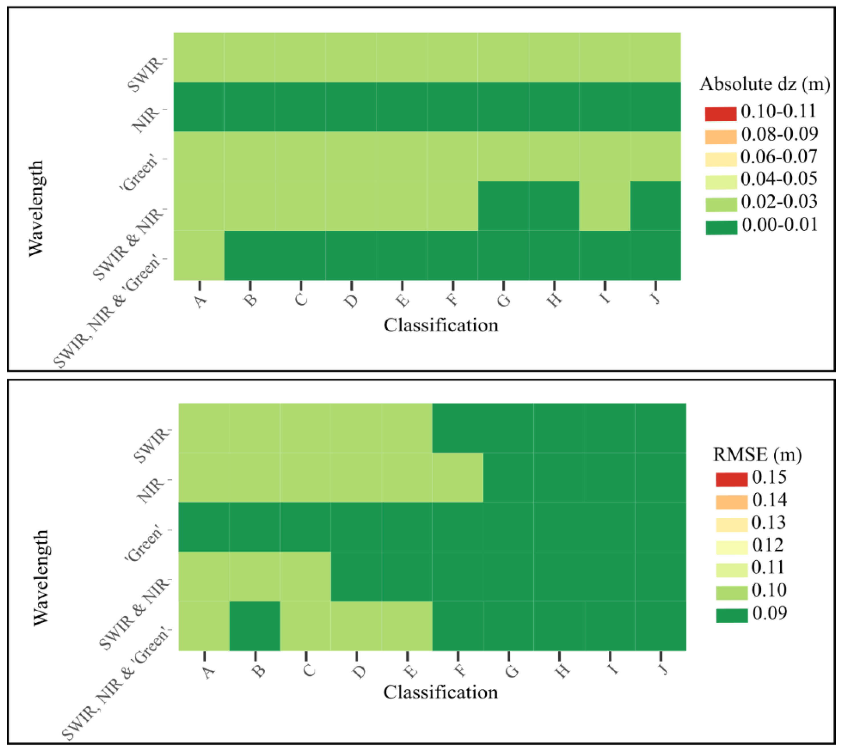
3.4. Differences between Field-Measured Elevation and Lidar Return Ground Classification in Taller Vegetative Regeneration Peatlands
3.5. Differences between Field-Measured Elevation and Lidar Return Ground Classification in Unburned Peatlands
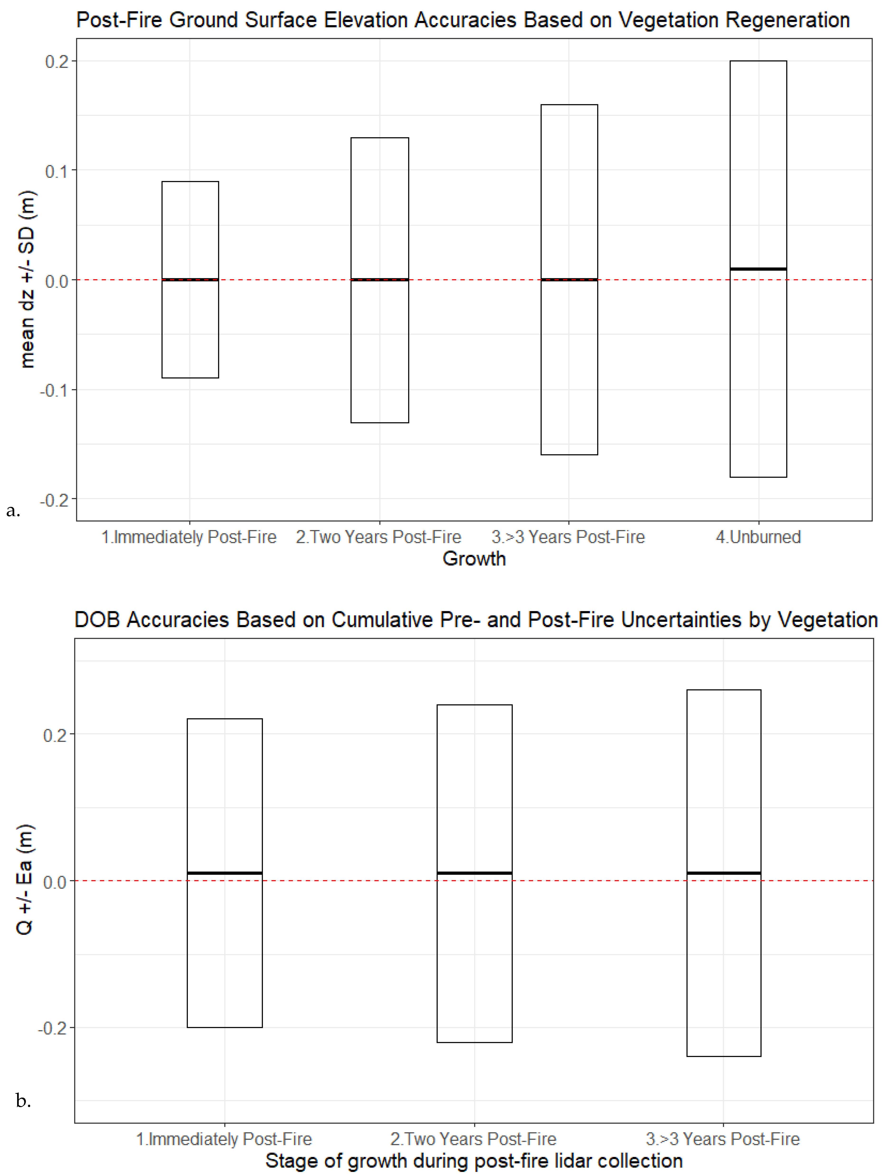
3.6. Expected Ground Surface Elevation Accuracies of Lidar Data in the Years following Wildland Fire
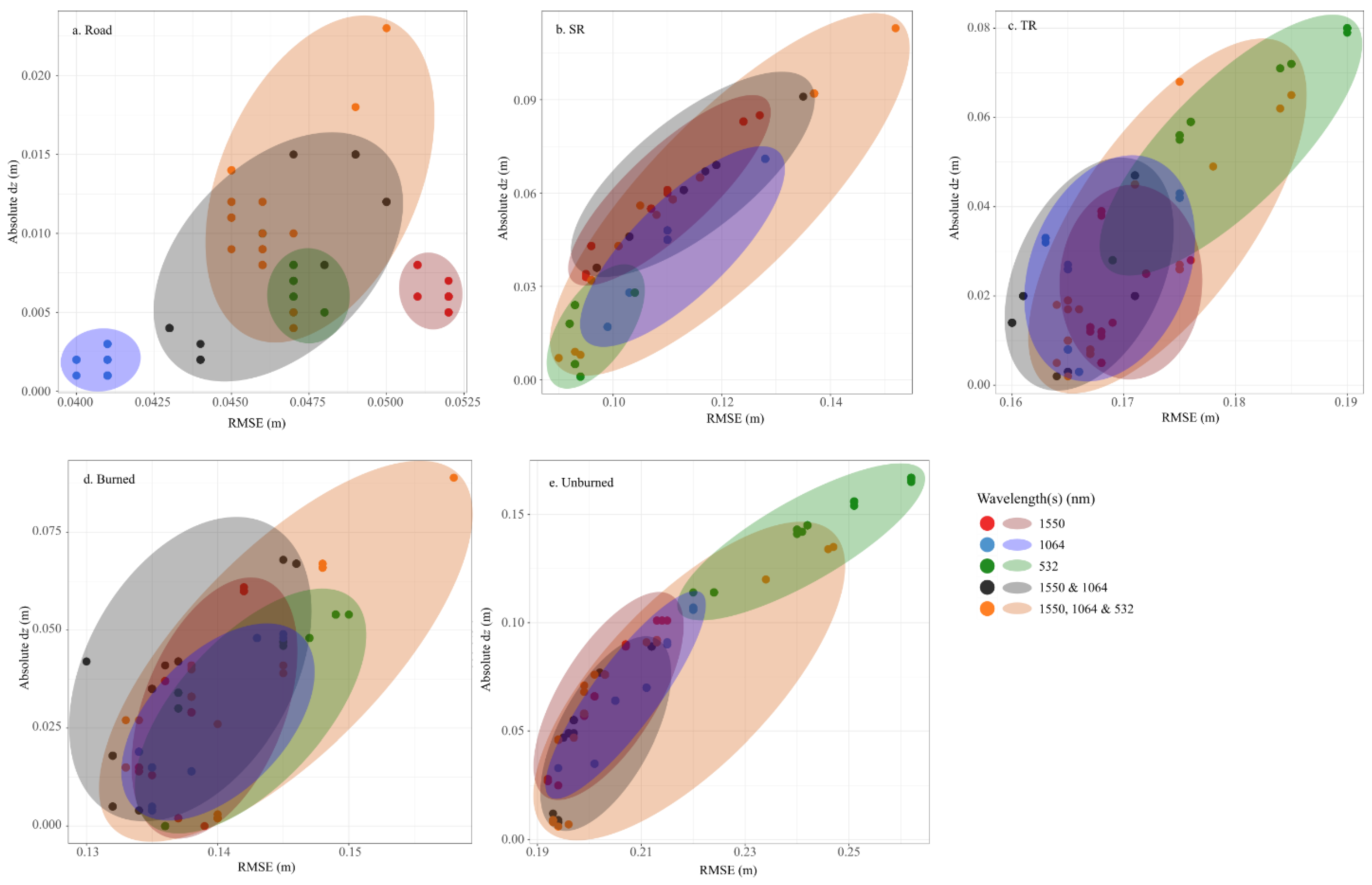
3.7. Wavelength Dependency of Ground Classification Accuracy as Varies by Vegetation Regeneration
4. Discussion
5. Conclusions
Supplementary Materials
Author Contributions
Funding
Data Availability Statement
Acknowledgments
Conflicts of Interest
References
- Frolking, S.; Roulet, N.T. Holocene radiative forcing impact of northern peatland carbon accumulation and methane emissions. Glob. Change Biol. 2007, 13, 1079–1088. [Google Scholar] [CrossRef]
- Yu, Z.C. Northern peatland carbon stocks and dynamics: A review. Biogeosciences 2012, 9, 4071–4085. [Google Scholar] [CrossRef] [Green Version]
- Flannigan, M.; Cantin, A.S.; De Groot, W.J.; Wotton, M.; Newbery, A.; Gowman, L.M. Global wildland fire season severity in the 21st century. For. Ecol. Manag. 2013, 294, 54–61. [Google Scholar] [CrossRef]
- Miller, C.A.; Benscoter, B.W.; Turetsky, M.R. The effect of long-term drying associated with experimental drainage and road construction on vegetation composition and productivity in boreal fens. Wetl. Ecol. Manag. 2015, 23, 845–854. [Google Scholar] [CrossRef]
- Walker, X.J.; Mack, M.C.; Johnstone, J.F. Stable carbon isotope analysis reveals widespread drought stress in boreal black spruce forests. Glob. Change Biol. 2015, 21, 3102–3113. [Google Scholar] [CrossRef]
- Kohlenberg, A.J.; Turetsky, M.R.; Thompson, D.K.; Branfireun, B.A.; Mitchell, C.P. Controls on boreal peat combustion and resulting emissions of carbon and mercury. Environ. Res. Lett. 2018, 13, 035005. [Google Scholar] [CrossRef] [Green Version]
- Van der Werf, G.R.; Randerson, J.T.; Giglio, L.; Collatz, G.J.; Mu, M.; Kasibhatla, P.S.; Morton, D.C.; DeFries, R.S.; Jin, Y.; van Leeuwen, T.T. Global fire emissions and the contribution of deforestation, savanna, forest, agricultural, and peat fires (1997–2009). Atmos. Chem. Phys. 2010, 10, 11707–11735. [Google Scholar] [CrossRef] [Green Version]
- Thompson, D.K.; Waddington, J.M. A Markov chain method for simulating bulk density profiles in boreal peatlands. Geoderma 2014, 232, 123–129. [Google Scholar] [CrossRef]
- Chasmer, L.E.; Hopkinson, C.D.; Petrone, R.M.; Sitar, M. Using multitemporal and multispectral airborne lidar to assess depth of peat loss and correspondence with a new active normalized burn ratio for wildfires. Geophys. Res. Lett. 2017, 44, 11851–11859. [Google Scholar] [CrossRef] [Green Version]
- Mickler, R.A.; Welch, D.P.; Bailey, A.D. Carbon emissions during wildland fire on a North American temperate peatland. Fire Ecol. 2017, 13, 34–57. [Google Scholar] [CrossRef]
- Lin, S.; Liu, Y.; Huang, X. Climate-induced Arctic-boreal peatland fire and carbon loss in the 21st century. Sci. Total Environ. 2021, 796, 148924. [Google Scholar] [CrossRef] [PubMed]
- Morison, M.; van Beest, C.; Macrae, M.; Nwaishi, F.; Petrone, R. Deeper burning in a boreal fen peatland 1-year post-wildfire accelerates recovery trajectory of carbon dioxide uptake. Ecohydrology 2021, 14, e2277. [Google Scholar] [CrossRef]
- Aguilar, F.J.; Mills, J.P. Accuracy assessment of LiDAR-derived digital elevation models. Photogramm. Rec. 2008, 23, 148–169. [Google Scholar] [CrossRef]
- Hokanson, K.J.; Lukenbach, M.C.; Devito, K.J.; Kettridge, N.; Petrone, R.M.; Waddington, J.M. Groundwater connectivity controls peat burn severity in the boreal plains: Groundwater controls peat burn severity. Ecohydrology 2016, 9, 574–584. [Google Scholar] [CrossRef]
- Whitman, E.; Parisien, M.A.; Holsinger, L.M.; Park, J.; Parks, S.A. A method for creating a burn severity atlas: An example from Alberta, Canada. Int. J. Wildland Fire 2020, 29, 995–1008. [Google Scholar] [CrossRef]
- Hudak, A.T.; Morgan, P.; Bobbitt, M.J.; Smith AM, S.; Lewis, S.A.; Lentile, L.B.; Robichaud, P.R.; Clark, J.T.; McKinley, R.A. The relationship of multispectral satellite imagery to immediate fire effects. Fire Ecol. 2007, 3, 64–90. [Google Scholar] [CrossRef]
- Hopkinson, C.; Chasmer, L.; Sass, G.; Creed, I.; Sitar, M.; Kalbfleisch, W.; Treitz, P. Vegetation class dependent errors in lidar ground elevation and canopy height estimates in a boreal wetland environment. Can. J. Remote Sens. 2005, 31, 191–206. [Google Scholar] [CrossRef]
- Ekhtari, N.; Glennie, C.; Fernandez-Diaz, J.C. Classification of airborne multispectral lidar point clouds for land cover mapping. IEEE J. Sel. Top. Appl. Earth Obs. Remote Sens. 2018, 11, 2068–2078. [Google Scholar] [CrossRef]
- Moudrý, V.; Klápště, P.; Fogl, M.; Gdulová, K.; Barták, V.; Urban, R. Assessment of LiDAR ground filtering algorithms for determining ground surface of non-natural terrain overgrown with forest and steppe vegetation. Measurement 2020, 150, 107047. [Google Scholar] [CrossRef]
- Andersen, H.E.; McGaughey, R.J.; Reutebuch, S.E. Estimating forest canopy fuel parameters using LIDAR data. Remote Sens. Environ. 2005, 94, 441–449. [Google Scholar] [CrossRef]
- McCarley, T.R.; Hudak, A.T.; Sparks, A.M.; Vaillant, N.M.; Meddens, A.J.; Trader, L.; Francisco, M.; Kreitler, J.; Boschetti, L. Estimating wildfire fuel consumption with multitemporal airborne laser scanning data and demonstrating linkage with MODIS-derived fire radiative energy. Remote Sens. Environ. 2020, 251, 112114. [Google Scholar] [CrossRef]
- Chen, Y.; Zhu, X.; Yebra, S.; Harris, N. Development of a predictive model for estimating forest surface fuel load in Australian eucalypt forests with LiDAR data. Environ. Model. Softw. 2017, 97, 61–71. [Google Scholar] [CrossRef]
- O’Neil, G.L.; Saby, L.; Band, L.E.; Goodall, J.L. Effects of LiDAR DEM smoothing and conditioning techniques on a topography-based wetland identification model. Water Resour. Res. 2019, 55, 4343–4363. [Google Scholar] [CrossRef]
- Millard, K.; Richardson, M. Wetland mapping with LiDAR derivatives, SAR polarimetric decompositions, and LiDAR–SAR fusion using a random forest classifier. Can. J. Remote Sens. 2013, 39, 290–307. [Google Scholar] [CrossRef]
- O’Neil, G.L.; Goodall, J.L.; Watson, L.T. Evaluating the potential for site-specific modification of LiDAR DEM derivatives to improve environmental planning-scale wetland identification using Random Forest classification. J. Hydrol. 2018, 559, 192–208. [Google Scholar] [CrossRef]
- Neugirg, F.; Kaiser, A.; Schmidt, J.; Becht, M.; Haas, F. Quantification, analysis and modelling of soil erosion on steep slopes using LiDAR and UAV photographs. Proc. Int. Assoc. Hydrol. Sci. 2015, 367, 51–58. [Google Scholar] [CrossRef] [Green Version]
- Escobar Villanueva, J.R.; Iglesias Martínez, L.; Pérez Montiel, J.I. DEM generation from fixed-wing UAV imaging and LiDAR-derived ground control points for flood estimations. Sensors 2019, 19, 3205. [Google Scholar] [CrossRef] [PubMed] [Green Version]
- Campbell, M.J.; Dennison, P.E.; Kerr, K.L.; Brewer, S.C.; Anderegg, W.R. Scaled biomass estimation in woodland ecosystems: Testing the individual and combined capacities of satellite multispectral and lidar data. Remote Sens. Environ. 2021, 262, 112511. [Google Scholar] [CrossRef]
- Schmid, K.A.; Hadley, B.C.; Wijekoon, N. Vertical accuracy and use of topographic LIDAR data in coastal marshes. J. Coast. Res. 2011, 27, 116–132. [Google Scholar] [CrossRef]
- Nelson, K.; Thompson, D.; Hopkinson, C.; Petrone, R.; Chasmer, L. Peatland-fire interactions: A review of wildland fire feedbacks and interactions in Canadian boreal peatlands. Sci. Total Environ. 2021, 769, 145212. [Google Scholar] [CrossRef]
- Downing, D.J.; Pettapiece, W.W. Natural Regions and Subregions of Alberta; Pub. No. T/852; Government of Alberta Publish: Edmonton, AB, Canada, 2006; 264p.
- Alberta Environment and Sustainable Resource Development (ESRD). Alberta Wetland Classification System; Water Policy Branch, Policy and Planning Division: Edmonton, AB, Canada, 2015. [Google Scholar]
- MNP LLP. A Review of the 2016 Horse River Wildfire; Forestry Division, Alberta Agriculture and Forestry: Edmonton, AB, Canada, 2017; Available online: https://www.alberta.ca/assets/documents/Wildfire-MNP-Report.pdf (accessed on 20 July 2021).
- Institute for Catastrophic Loss Reduction. Fort McMurray Wildfire: Learning from Canada’s Costliest Disaster; Institute for Catastrophic Loss Reduction: Toronto, ON, Canada, 2019; p. 9. Available online: https://www.zurichcanada.com/-/media/project/zwp/canada/docs/english/weather/fort-mcmurray-report_canada.pdf (accessed on 16 May 2021).
- Csanyi, N.; Toth, C.K. Improvement of lidar data accuracy using lidar-specific ground targets. Photogramm. Eng. Remote Sens. 2007, 73, 385–396. [Google Scholar] [CrossRef] [Green Version]
- Axelsson, P. DEM generation from laser scanner data using adaptive TIN models. Int. Arch. Photogramm. Remote Sens. 2000, 33, 110–117. [Google Scholar]
- GeoCue Group. TerraScan Ground Parameters. 2020. Available online: https://support.geocue.com/terrascan-ground-filter-parameters/ (accessed on 10 February 2021).
- Terrasolid Ltd. TerraScan User Guide. Terrasolid Ltd., Batch Processing Reference > Classification Routines > Points > Ground. 2021. Available online: https://terrasolid.com/guides/tscan/crground.html (accessed on 10 November 2021).
- Rapidlasso GmbH. Lasground_New README. 2021. Available online: https://lastools.github.io/download/lasground_new_README.txt (accessed on 5 December 2021).
- ASPRS. ASPRS Guidelines: Vertical Accuracy Reporting for Lidar Data Version 1.0; American Society for Photogrammetry and Remote Sensing Lidar Committee (PAD): Baton Rouge, LA, USA, 2004. [Google Scholar]
- Pourali, S.; Arrowsmith, C.; Chrisman, N.; Matkan, A. Vertical accuracy assessment of LiDAR ground points using minimum distance approach. In Proceedings of the Research Locate 14, Canberra, Australia, 7–9 April 2014. [Google Scholar]
- Maune, D.; Black, T.; Constance, E. DEM user requirements. In Digital Elevation Model Technologies and Applications: The DEM Users Manual, 2nd ed.; American Society for Photogrammatry and Remote Sensing: Bethesda, MD, USA, 2007; pp. 449–473. [Google Scholar]
- Goulden, T.; Hopkinson, C.; Jamieson, R.; Sterling, S. Sensitivity of DEM, slope, aspect and watershed attributes to LiDAR measurement uncertainty. Remote Sens. Environ. 2016, 179, 23–35. [Google Scholar] [CrossRef]
- GeoCue Group. Control Point Statistics in TerraScan: TerraScan, Versions 002.001 and Above. 2017. Available online: https://support.geocue.com/wp-content/uploads/2017/03/Control-Point-Statistics-in-TerraScan.pdf (accessed on 10 February 2021).
- Carlisle, B.H. Modelling the spatial distribution of DEM error. Trans. GIS 2005, 9, 521–540. [Google Scholar] [CrossRef]
- Goulden, T.; Hopkinson, C. The forward propagation of integrated system component errors within airborne lidar data. Photogramm. Eng. Remote Sens. 2010, 76, 589–601. [Google Scholar] [CrossRef]
- Goulden, T.; Hopkinson, C. Mapping simulated error due to terrain slope in airborne lidar observations. Int. J. Remote Sens. 2014, 35, 7099–7117. [Google Scholar] [CrossRef]
- Hopkinson, C.; Chasmer, L.E.; Zsigovics, G.; Creed, I.F.; Sitar, M.; Treitz, P.; Maher, R.V. Errors in LIDAR ground elevations and wetland vegetation height estimates. Int. Arch. Photogramm. Remote Sens. Spat. Inf. Sci. 2004, 36, 108–113. [Google Scholar]
- Brubaker, K.M.; Myers, W.L.; Drohan, P.J.; Miller, D.A.; Boyer, E.W. The use of LiDAR terrain data in characterizing surface roughness and microtopography. Appl. Environ. Soil Sci. 2013, 2013, 891534. [Google Scholar] [CrossRef]
- Tinkham, W.T.; Smith, A.M.; Hoffman, C.; Hudak, A.T.; Falkowski, M.J.; Swanson, M.E.; Gessler, P.E. Investigating the influence of LiDAR ground surface errors on the utility of derived forest inventories. Can. J. For. Res. 2012, 42, 413–422. [Google Scholar] [CrossRef]
- Hopkinson, C.; Chasmer, L.; Gynan, C.; Mahoney, C.; Sitar, M. Multisensor and multispectral lidar characterization and classification of a forest environment. Can. J. Remote Sens. 2016, 42, 501–520. [Google Scholar] [CrossRef]
- Okhrimenko, M.; Coburn, C.; Hopkinson, C. Multispectral lidar: Radiometric calibration, canopy spectral reflectance, and vegetation vertical SVI profiles. Remote Sens. 2019, 11, 1556. [Google Scholar] [CrossRef] [Green Version]
- Reddy, A.D.; Hawbaker, T.J.; Wurster, F.; Zhu, Z.; Ward, S.; Newcomb, D.; Murray, R. Quantifying soil carbon loss and uncertainty from peatland wildfire using multi-temporal LiDAR. Remote Sens. Environ. 2015, 170, 306–316. [Google Scholar] [CrossRef]
- Gerrand, S.; Aspinall, J.; Jensen, T.; Hopkinson, C.; Collingwood, A.; Chasmer, L. Partitioning carbon losses from fire combustion in a montane valley, Alberta Canada. For. Ecol. Manag. 2021, 496, 119435. [Google Scholar] [CrossRef]
- Benscoter, B.W.; Greenacre, D.; Turetsky, M.R. Wildland fire as a key determinant of peatland microtopography. Can. J. For. Res. 2015, 45, 1132–1136. [Google Scholar] [CrossRef]
- Kasischke, E.S.; Johnstone, J.F. Variation in postfire organic layer thickness in a black spruce forest complex in interior Alaska and its effects on soil temperature and moisture. Can. J. For. Res. 2005, 35, 2164–2177. [Google Scholar] [CrossRef] [Green Version]
- Boby, L.A.; Schuur, E.A.; Mack, M.C.; Verbyla, D.; Johnstone, J.F. Quantifying fire severity, carbon, and nitrogen emissions in Alaska’s boreal forest. Ecol. Appl. 2010, 20, 1633–1647. [Google Scholar] [CrossRef]


| Ground Classification | Max Building Size | Terrain Angle | Iteration Angle | Iteration Distance | Reduce Iteration Angle When Edge Length< | Stop Triangulation When Edge Length< |
|---|---|---|---|---|---|---|
| 1 | 60 | 50 | 6 | 1.4 | 5 | - |
| 2 | 60 | 55 | 6 | 1.4 | 5 | - |
| 3 | 60 | 60 | 6 | 1.4 | 5 | - |
| 4 | 60 | 65 | 6 | 1.4 | 5 | - |
| 5 | 60 | 70 | 6 | 1.4 | 5 | - |
| 6 | 60 | 75 | 6 | 1.4 | 5 | - |
| 7 | 60 | 80 | 6 | 1.4 | 5 | - |
| 8 | 60 | 88 | 6 | 1.4 | 5 | - |
| 9 | 60 | 88 | 2 | 1.4 | 5 | - |
| 10 | 60 | 88 | 2 | 0.5 | 5 | - |
| 11 | 60 | 88 | 2 | 1 | 5 | - |
| 12 | 60 | 88 | 2 | 1.5 | 5 | - |
| 13 | 60 | 88 | 2 | 2 | 5 | - |
| 14 | 60 | 88 | 5 | 1.4 | 5 | - |
| 15 | 60 | 88 | 5 | 0.5 | 5 | - |
| 16 | 60 | 88 | 5 | 1 | 5 | - |
| 17 | 60 | 88 | 5 | 1.5 | 5 | - |
| 18 | 60 | 88 | 5 | 2 | 5 | - |
| 19 | 60 | 88 | 10 | 1.4 | 5 | - |
| 20 | 60 | 88 | 10 | 0.5 | 5 | - |
| 21 | 60 | 88 | 10 | 1 | 5 | - |
| 22 | 60 | 88 | 10 | 1.5 | 5 | - |
| 23 | 60 | 88 | 10 | 2 | 5 | - |
| 24 | 60 | 88 | 15 | 1.4 | 5 | - |
| 25 | 60 | 88 | 15 | 0.5 | 5 | - |
| 26 | 60 | 88 | 15 | 1 | 5 | - |
| 27 | 60 | 88 | 15 | 1.5 | 5 | - |
| 28 | 60 | 88 | 15 | 2 | 5 | - |
| 29 | 60 | 88 | 15 | 1.5 | - | - |
| 30 | 60 | 88 | 15 | 1.5 | 1 | - |
| 31 | 60 | 88 | 15 | 1.5 | 2 | - |
| 32 | 60 | 88 | 15 | 1.5 | 10 | - |
| 33 | 60 | 88 | 15 | 1.5 | 5 | 0.5 |
| 34 | 60 | 88 | 15 | 1.5 | 5 | 2 |
| 35 | 60 | 88 | 15 | 1.5 | 5 | 5 |
| 36 | 60 | 88 | 15 | 1.5 | 5 | 0.25 |
| Ground Classification | Refinement | Bulge (m) | Step Size (m) | Subgrid for Initial Ground Points | |
|---|---|---|---|---|---|
| A | Nature | Default | 0.5 | 5 | =step size |
| B | Nature | Fine | 0.5 | 5 | Default granularity × 4 |
| C | Nature | Extra Fine | 0.5 | 5 | Fine granularity × 4 |
| D | Nature | Ultra-Fine | 0.5 | 5 | Extra Fine granularity × 4 |
| E | Nature | Hyper Fine | 0.5 | 5 | Ultra-Fine granularity × 4 |
| F | Wilderness | Default | 0.3 | 3 | =step size |
| G | Wilderness | Fine | 0.3 | 3 | Default granularity × 4 |
| H | Wilderness | Extra Fine | 0.3 | 3 | Fine granularity × 4 |
| I | Wilderness | Ultra-Fine | 0.3 | 3 | Extra Fine granularity × 4 |
| J | Wilderness | Hyper Fine | 0.3 | 3 | Ultra-Fine granularity × 4 |
Publisher’s Note: MDPI stays neutral with regard to jurisdictional claims in published maps and institutional affiliations. |
© 2022 by the authors. Licensee MDPI, Basel, Switzerland. This article is an open access article distributed under the terms and conditions of the Creative Commons Attribution (CC BY) license (https://creativecommons.org/licenses/by/4.0/).
Share and Cite
Nelson, K.; Chasmer, L.; Hopkinson, C. Quantifying Lidar Elevation Accuracy: Parameterization and Wavelength Selection for Optimal Ground Classifications Based on Time since Fire/Disturbance. Remote Sens. 2022, 14, 5080. https://doi.org/10.3390/rs14205080
Nelson K, Chasmer L, Hopkinson C. Quantifying Lidar Elevation Accuracy: Parameterization and Wavelength Selection for Optimal Ground Classifications Based on Time since Fire/Disturbance. Remote Sensing. 2022; 14(20):5080. https://doi.org/10.3390/rs14205080
Chicago/Turabian StyleNelson, Kailyn, Laura Chasmer, and Chris Hopkinson. 2022. "Quantifying Lidar Elevation Accuracy: Parameterization and Wavelength Selection for Optimal Ground Classifications Based on Time since Fire/Disturbance" Remote Sensing 14, no. 20: 5080. https://doi.org/10.3390/rs14205080